Strength function: convergence of the Mittag-Leffler expansion

We saw in the strength_function.ipynb notebook that the strength function (SF) can be approximated by using a Mittag-Leffler expansion (MLE) of the Green’s function. In this notebook, we’ll see how the MLE of the SF converges to the exact result when the number of resonant couples used is increased.

Initialization

This part very similar to the previous notebook, but don’t forget to run the cells before jumping to the next section!

Import some modules and classes

# Make the notebook aware of some of the SiegPy module classes
from siegpy import SWPBasisSet, Rectangular, Gaussian, SWPotential
# Other imports
import numpy as np
import matplotlib.pyplot as plt

Create a basis-set made of Siegert states only

siegerts = SWPBasisSet.from_file("siegerts.dat", nres=25)

Define test functions to evaluate the strength function

l = siegerts.potential.width  # width of the potential
x_c = 0.0  # Center of the test functions
a = l/2  # Width of the rectangular function
sigma = l/20  # Width of the Gaussian
test_gauss = Gaussian(sigma, x_c)  # Gaussian test function
test_rect = Rectangular.from_width_and_center(a, x_c)  # Rectangular test function

Create the grid of wavenumbers where the strength function is evaluated

It is not mandatory to keep the same grid as for the continuum states, and it is strongly advised to decrease this number as much as possible to save computation time, since an integration over all continuum states is performed for each point in this grid, that only defines the grid used for plotting.

h_k = 0.05  # Grid-step for plotting
k_max = 10  # Maximal wavenumber for plotting
kgrid = np.arange(h_k, k_max, h_k)

Tests of convergence of the MLE of the strength function

We present the evolution of the MLE of the strength function as a function of the number of resonant couples included in the approximated Green’s function.

We will see that with only a few resonant couples considered, it is possible to get a correct evaluation of the strength function on a rather large range of wavenumber

Case 1: Gaussian test function

The first step corresponds in evaluating the strength function for basis sets of increasing size. To that end, the contribution of all the bound and anti-bound states is evaluated separately (stored in b_a_MLE_g), while the strength function associated to each resonant couple is stored in the list r_MLE_g.

# Create basis sets with bound and antibound states, with resonant states
# and with anti-resonant states.
bnds_abnds = siegerts.bounds + siegerts.antibounds
res = siegerts.resonants
ares = siegerts.antiresonants

# Contribution of the bound and anti-bound states to the MLE of the SF
b_a_MLE_g = bnds_abnds.MLE_strength_function(test_gauss, kgrid)
# Contribution of each resonant couple to the MLE of the SF
r_MLE_g   = [SWPBasisSet(states=[res[i], ares[i]]).MLE_strength_function(test_gauss, kgrid) for i in range(len(res))]

After some matplotlib manipulation, you get the following plot:

#Plot the reference, with all siegert states
plt.plot(kgrid, b_a_MLE_g + sum(r_MLE_g), color='k', lw=5,
         label='$N_{res}$ = '+str(len(res)))
#Plot the first: bound states contribution only
colors = ['#0c2c84', '#1d91c0', '#7fcdbb', '#c7e9b4']
plt.plot(kgrid, b_a_MLE_g, color=colors[0], label='$N_{res}$ = 0')
#Plot the rest
for i in [2, 4, 6]:
    plt.plot(kgrid, b_a_MLE_g + sum(r_MLE_g[:i]),
             color=colors[i//2], label='$N_{res}$ = '+str(i))
plt.xlabel("$k$")
plt.ylabel("$R(k)$")
plt.title('Gaussian test function')
plt.legend()
plt.show()

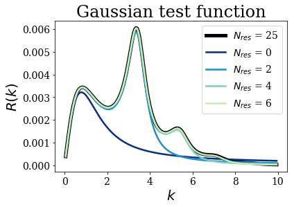
As you can see, using a handful of resonant couples leads to almost converged result over a rather large range of wavenumbers. Remember that the exact result would require a rather dense basis set of continuum states to reach the same convergence, while the physical information on the resonances would be absent. The approximation of the Green’s function by Siegert states is very promising.

Case 2: rectangular test function

You can easily repeat that same study for a rectangular test function:

# Contribution of the bound and anti-bound states to the MLE of the SF
b_a_MLE_r = bnds_abnds.MLE_strength_function(test_rect, kgrid)
# Contribution of each resonant couples to the MLE of the SF
r_MLE_r   = [SWPBasisSet([res[i], ares[i]]).MLE_strength_function(test_rect, kgrid) for i in range(len(res))]

#Plot the reference, with all siegert states
plt.plot(kgrid, b_a_MLE_r + sum(r_MLE_r), color='k', lw=5,
         label='$N_{res}$ = '+str(len(res)))
#Plot the first: bound states contribution only
colors = ['#0c2c84', '#1d91c0', '#41b6c4', '#7fcdbb', '#c7e9b4']
plt.plot(kgrid, b_a_MLE_r, color=colors[0], label='$N_{res}$ = 0')
#Plot the rest
for i in [2, 4, 6, 8]:
    plt.plot(kgrid, b_a_MLE_r + sum(r_MLE_r[:i]),
             color=colors[i//2], label='$N_{res}$ = '+str(2*i))
plt.xlabel("$k$")
plt.ylabel("$R(k)$")
plt.title('Rectangular test function')
plt.legend()
plt.show()

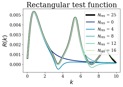
Note that, even if the strength function erroneously reaches negative values, the position and the shape of the first peaks are still very well reproduced by only a few resonant couples.