Virial operators

We saw in previous notebooks that the expectation values of the virial operators were able to discriminate the Siegert states from any other type of states. All the previous notebooks only used one type of virial operator, but there are two definitions in SiegPy. The goal of this notebook is to present the second type of virial operator, and how it compares to the default one.

Initialization

The initialization is simple: we only import the useful modules and classes and then define a potential (which is a 1D Square-Well Potential discretized over a space grid).

Import some modules and classes

from siegpy import (Hamiltonian, SWPotential, ErfKGCoordMap,
                    SWPBasisSet)
import numpy as np

Define a potential

# The potential is read from a file...
siegerts = SWPBasisSet.from_file("siegerts.dat")
pot = siegerts.potential
# ... and then discretized over a grid
l = pot.width
xmax = 7.5
xgrid = np.linspace(-xmax, xmax, 501)
pot.grid = xgrid

Choosing the virial operator

The default virial operator gives one (and only one) value. It actually measures if the position-momentum commutator is correctly evaluated when applied to a given eigenstate \(\varphi\), i.e., it is such that \(\left\langle \varphi | [\hat{X}, \hat{P}] | \varphi \right\rangle = i \left\langle \varphi | \varphi \right\rangle\). It is referred to as the Generalized Coplex Virial Theorem (GCVT).

The other is available for SmoothExtCoordMap instances only, for which a virial operator \(\hat{W_\xi} = \frac{\text{d} \hat{H}}{\text{d} \xi}\) per parameter \(\xi\) (here the angle \(\theta\), the inflexion point \(x_0\) and the sharpness \(\lambda\)) is defined (\(\hat{H}\) is the Hamiltonian considered). These virial operators measure the stability of each eigenvalue with respect to a given parameter change. Each virial operator then gives rise to one virial expectation value per parameter, namely \(v_\xi = \left\langle \varphi | \hat{W_\xi} | \varphi \right\rangle\). These three values are finally mapped into one final virial value \(v\) by using the following equation \(v = \sum_{\xi \in [\theta, x_0, \lambda]} | v_\xi |^2\).

The choice of the type of virial operator used is done while initializing the coordinate mapping, by setting the optional parameter GCVT either to True or False.

# Initial parameters
theta = 0.6
x0 = 6.0
lbda = 1.5
# Default virial operator: GCVT=True
cm_1 = ErfKGCoordMap(theta, x0, lbda, grid=xgrid)
# Other type of virial operator: GCVT=False
cm_2 = ErfKGCoordMap(theta, x0, lbda, grid=xgrid, GCVT=False)

Comparing the virial operators

Define and solve two Hamiltonians

One Hamitonian per type of virial operator is defined and then solved.

ham_1 = Hamiltonian(pot, cm_1)
ham_2 = Hamiltonian(pot, cm_2)

basis_1 = ham_1.solve()
basis_2 = ham_2.solve()

Plot the energies

The plot_energies method of the basis sets allows to see how the virial values are distributed over the energy spectrum. Note that both basis sets are made of the same states: only their associated virial expecation values are different.

basis_1.plot_energies()
basis_2.plot_energies()

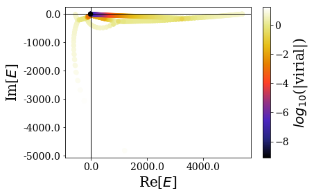
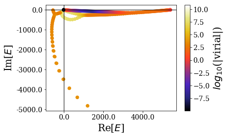
As you can see, the distribution of the virial expectation values differ greatly between both virial operators:

• The range of virial values is much larger for the second type of virial operator.
• Most importantly, the resonant states with the lowest virial expectation values are very different: for the default virial operator, the lowest energy resonant states have the lowest virial expecation values, while a maximum value is reached far away from the 0 energy for the second type of virial operator:

for state in basis_2[:12]:
    print(state.energy, state.virial)

(-9.79608688842+4.10071842408e-14j) 1.14043002476e-10
(-9.18591925228-3.37715726075e-14j) 6.82940051154e-10
(-8.17464337214+4.21396607849e-14j) 3.18687656971e-09
(-6.77260946384+2.61389816265e-14j) 1.80012213375e-08
(1346.81487901-70.0870431848j) 1.33383817064e-07
(1309.64971825-68.7242290591j) 1.43891530556e-07
(1384.60670122-71.4821234553j) 1.53861789445e-07
(-4.99980420562-1.44406627299e-11j) 1.64899673628e-07
(1273.09631514-67.3909816174j) 1.88483607705e-07
(1423.04138812-72.9122466557j) 2.49175889283e-07
(1237.1410264-66.0847007287j) 2.74099981855e-07
(1201.77142174-64.80290349j) 4.14687367264e-07

for state in basis_1[:12]:
    print(state.energy, state.virial)

(-9.79608688842+4.10071842408e-14j) 7.97704509282e-10
(-9.18591925228-3.37715726075e-14j) 3.17680862089e-09
(-8.17464337214+4.21396607849e-14j) 7.08919431335e-09
(-6.77260946384+2.61389816265e-14j) 1.24276304178e-08
(-4.99980420562-1.44406627299e-11j) 1.89478510917e-08
(-2.90018622708-6.14397704638e-09j) 2.59530586763e-08
(-0.626085020601+7.33146819469e-06j) 4.82648903582e-08
(1.87104013925-0.944793379409j) 5.54727310476e-08
(5.52735942521-1.73866474126j) 6.89860589855e-08
(9.68066945927-2.4642996033j) 8.75410584435e-08
(14.3306084456-3.18636534093j) 1.08537828898e-07
(19.4768829199-3.92000638226j) 1.31971445351e-07

Zooming in more closely to the 0 energy, the differences can be more easily spotted in this energy range:

basis_1.plot_energies(xlim=(-10, 50), ylim=(-7.5, 0.5))
basis_2.plot_energies(xlim=(-10, 50), ylim=(-7.5, 0.5))

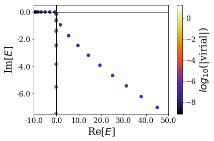
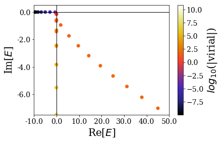
The variation of the bound state virial values is much larger for the second type of virial operator, and it makes it more difficult (if not impossible) to say that the first resonant states can be sorted out from the rest of the eigenstates by their virial expectation value.

Conclusion

The default virial operator, measuring how the position-momentum commutator is correctly evaluated by the eigenstates, is better than the other one when it comes to separate the Siegert states from the rest of the numerical eigenstates. It is therefore advised to keep using this default virial operator.