Multiple Gaussian potentials

In this notebook, we will present another type of potentials, made of Gaussian functions. There will be two or four Gaussian functions used to define each potential.

The initial potential to be studied in this notebook is made of two Gaussian wells, and we will see the influence of two parameters on the obtained spectra:

• the addition of two Gaussian barriers (one on each side of the two initial Gaussian wells)
• the distance between the two Gaussian wells

Initialization

The same initialization is required than for the notebook about the Woods-Saxon potential, the two difference being that two other classes of symbolic potentials are imported: TwoGaussianPotential and FourGaussianPotential.

import numpy as np
import matplotlib.pyplot as plt
import matplotlib.colors
from matplotlib import cm
from siegpy import (Hamiltonian, ErfKGCoordMap, BasisSet,
                    TwoGaussianPotential, FourGaussianPotential)

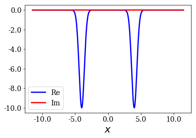
Two identical Gaussian wells

The first potential is made of two identical Gaussian wells that are not too broadly separated:

# Define a grid
xmax = 11.5
xgrid = np.linspace(-xmax, xmax,1201)
# Define a depth, sigma and center for the Gaussian potential
sigma = 0.4
xc = 2
V0 = 10
# Define a Potential with two Gaussian functions
sym_pot1 = TwoGaussianPotential(sigma, -xc, -V0, sigma, xc, -V0, grid=xgrid)
sym_pot1.plot()

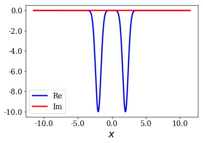
The depth and sigma defined here will be used throughout this notebook.

The potential is then used to define a Hamiltonian, that is finally solved in order to create a basis set:

cm_g = ErfKGCoordMap(0.6, 10.0, 1.0)
ham1 = Hamiltonian(sym_pot1, cm_g)
basis1 = ham1.solve(max_virial=10**(-6))

Finally, let us show some plots:

# Definition of all the parameters to get consistent plots for
# all the potentials considered throughout this notebook
re_e_max = 15
im_e_min = -6
im_k_max = np.sqrt(2*V0)
re_k_max = np.sqrt(2*re_e_max)
re_e_lim = (-V0, re_e_max)
im_e_lim = (im_e_min, -im_e_min/30)
re_k_lim = (-re_k_max/30, re_k_max)
im_k_lim = (-im_k_max, im_k_max)
# Plot the energies, wavenumbers and some eigenstates of the potential
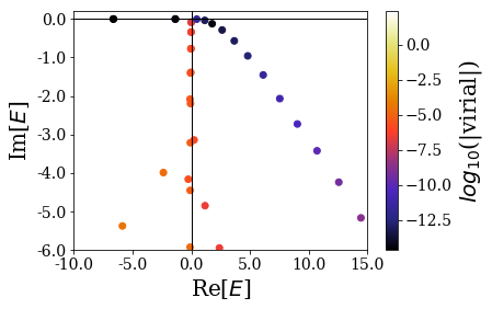
basis1.plot_energies(xlim=re_e_lim, ylim=im_e_lim)
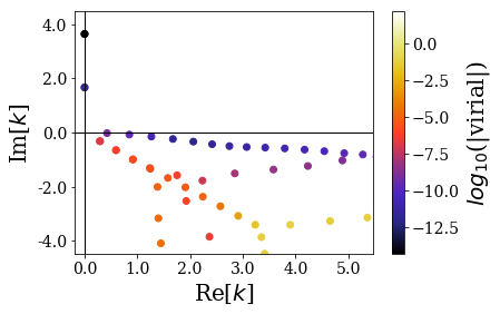
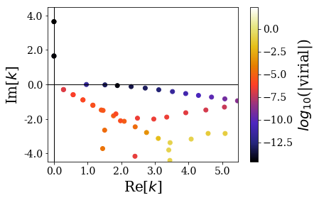
basis1.plot_wavenumbers(xlim=re_k_lim, ylim=im_k_lim)
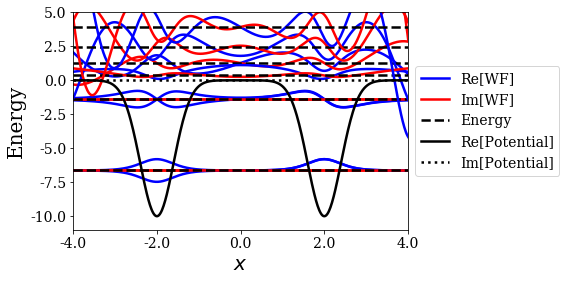
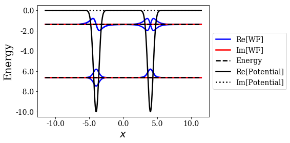
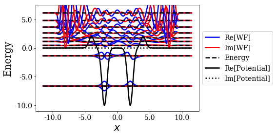
basis1.plot_wavefunctions(nres=4, xlim=(-4, 4), ylim=(-V0-1, 5))

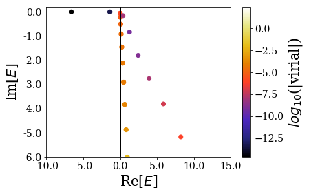
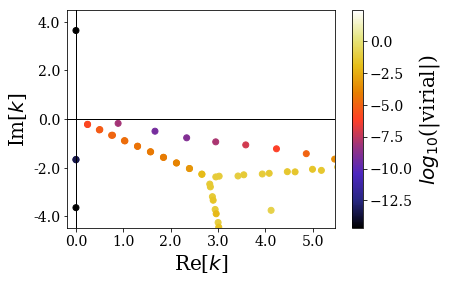
Both bound and resonant states are found and are separable from the rest of the states, even if the resonant states virial values are rather high for the resonant states.

Note that the bound states actually are degenerate: the separation between both Gaussian wells is large enough to avoid a large overlap of the bound states wavefunctions of each Gaussian well. It is easy to see that by using simple linear combinations (addition and subtraction) of these degenerate bound states wavefunctions of a given energy, one gets the bound states of each Gaussian well.

Some resonant states can also be separated from the rotated continuum states thanks to their virial values, even though only few of them are found in this case. The first resonant state has a rather long lifetime (proportional to the inverse of its imaginary part (in absolute value)), while the other next resonant states are associated to decreasing lifetimes.

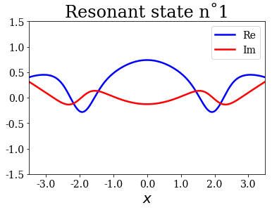
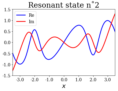
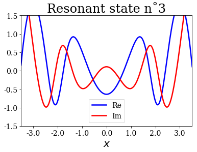
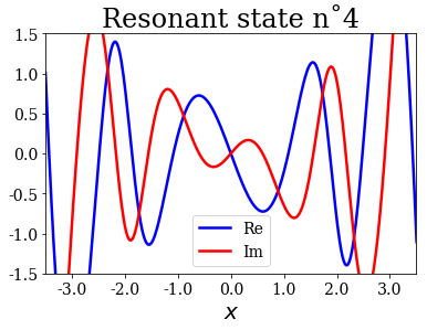
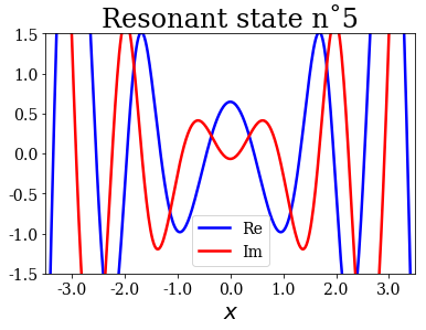
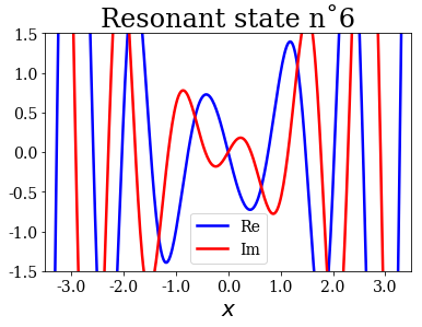
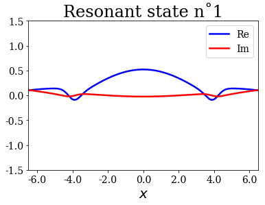
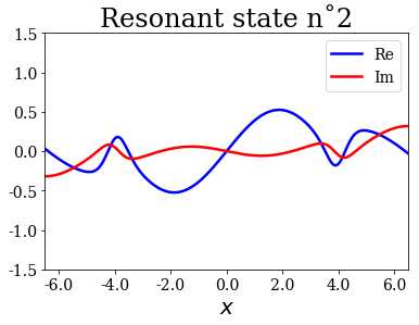
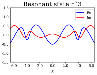
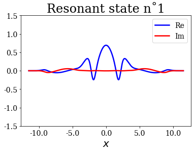
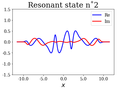
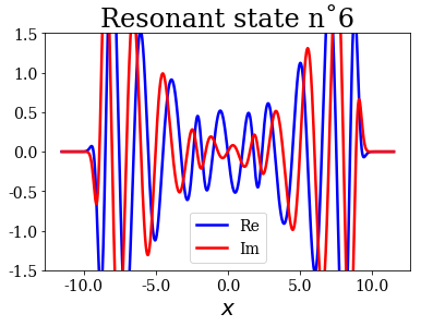
It is worth noting that the resonant states wavefunctions have anti-nodes centered between both Gaussian wells, and the number of nodes in this region keeps increasing, starting from one anti-node for the first resonant state. This is more clearly presented below:

# Sort the resonant states by increasing real energy
res = basis1.resonants.states
res.sort(key=lambda x: x.energy.real)
# Plot each one of them
for i, state in enumerate(res):
    xmax = 3.5; ymax = 1.5
    tit = "Resonant state n˚{}".format(i+1)
    state.plot(title=tit, xlim=(-xmax, xmax), ylim=(-ymax, ymax))

Increase of the separation between both potentials

Let us consider a similar case, wit the same Gaussian wells, the main difference being that they are separated by a larger distance, that should lead to even less overlap between the bound states of each potential:

# Center of the new Gaussian wells
xc2 = 4
# Definition of the new potential
sym_pot2 = TwoGaussianPotential(sigma, -xc2, -V0, sigma, xc2, -V0, grid=xgrid)
sym_pot2.plot()

As usual, this potential is used to define a Hamiltonian, which is in turn solved, so that a basis set is created:

ham2 = Hamiltonian(sym_pot2, cm_g)
basis2 = ham2.solve(max_virial=10**(-8.7))

The same plots are done for this new potential:

basis2.plot_energies(xlim=re_e_lim, ylim=im_e_lim)
basis2.plot_wavenumbers(xlim=re_k_lim, ylim=im_k_lim)
basis2.plot_wavefunctions(nres=0)

The spectrum of bound states is the same as in the previous case, while the spectrum of resonant states is very different: the number of resonant states in the same energy range is larger and they are associated to larger lifetimes. This shows that it is easier to have low energy resonant states when the distance between two potential wells is increased. This effect is actually similar to what is known for the bound states of a potential well of increasing width: the energies of the low energy bound states tend to get closer to each other. The same phenomenon occurs here for the resonant states: it is as if they were trapped between the two potential wells, that effectively act as a single potential well for the resonant states.

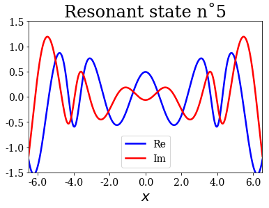
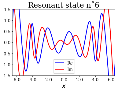
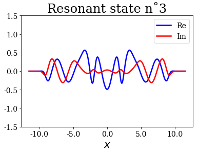
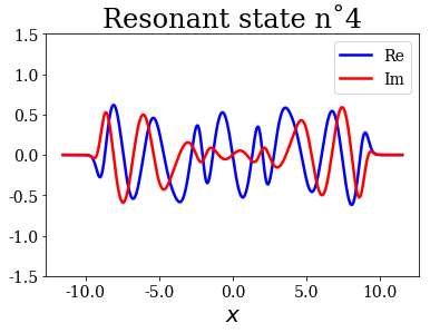
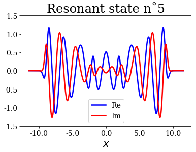
The resonant wavefunctions follow the same pattern as the one found for the previous potential, with an increasing number of anti-nodes between both wells for the resonant states of increasing energy:

# Sort the resonant states by increasing real energy
res = basis2.resonants.states
res.sort(key=lambda x: x.energy.real)
# Plot each one of them
for i, state in enumerate(res[:6]):
    xmax = 6.5; ymax = 1.5
    tit = "Resonant state n˚{}".format(i+1)
    state.plot(title=tit, xlim=(-xmax, xmax), ylim=(-ymax, ymax))

Gaussian barriers around the two Gaussian wells

Let us finally consider a last case where a potential barrier is added on each side of the initial Gaussian wells. These barriers are Gaussian functions that have the same center as the Gaussian wells used to define the previous potential:

# Depth of the extra Gaussian barriers
V1 = 0.2 * V0
# Definition of the potential
sym_pot3 = FourGaussianPotential(sigma, -xc2, V1, sigma, -xc, -V0,
                                 sigma, xc, -V0, sigma, xc2, V1, grid=xgrid)
sym_pot3.plot()

A Hamiltonian is created from this potential, and solved to give a basis set:

ham3 = Hamiltonian(sym_pot3, cm_g)
basis3 = ham3.solve(max_virial=10**(-9))

The basis set is then used to create some plots:

basis3.plot_energies(xlim=re_e_lim, ylim=im_e_lim)
basis3.plot_wavenumbers(xlim=re_k_lim, ylim=im_k_lim)
basis3.plot_wavefunctions(nres=7, ylim=(-11, 7.5))

Again, the bound states and the resonant states can easily be separated from the rest of the resonant states. The virial values are even larger for the resonant states. Again, the bound states are degenerate, and they are the same as the ones found for the other potentials without the barriers.

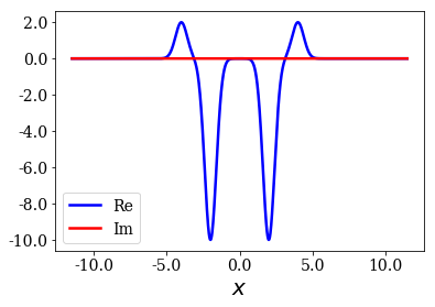
The first three resonant states can be considered as quasi-bound, in the sense that their lifetime is very large and because their energy is below the maximum of the Gaussian barriers. Also note how their wavefunction does not tend to diverge, especially compared to the other resonant states of higher energy, which are nothing but the same type of resonant states we used to find for other potentials. Also note how the number of anti-nodes of the resonant states wavefunction still follows the same increase when the resonant energy is increased. The presence of the barrier does not affect this property of the resonant states, whether they are quasi-bound or not. The first resonant states wavefunctions are presented below:

# Sort the resonant states by increasing real energy
res = basis3.resonants.states
res.sort(key=lambda x: x.energy.real)
# Plot each one of them
for i, state in enumerate(res[:6]):
    xmax = 9.5; ymax = 1.5
    tit = "Resonant state n˚{}".format(i+1)
    state.plot(title=tit, ylim=(-ymax, ymax))

Comparison of the eigenstates

To get a clearer view on the spectra obtained with the various potentials, the same function as for the case of the Woods-Saxon potential is defined:

def scatter_plot(data_kwd, basissets, xlim=None, ylim=None, title=None,
                 file_save=None, show_unknown=False):
    # Object-oriented plots
    fig = plt.figure()
    ax = fig.add_subplot(111)
    # Add the real and imaginary axes
    ax.axhline(0, color='black', lw=1)  # black line y=0
    ax.axvline(0, color='black', lw=1)  # black line x=0
    # Define the min and max values of the virial, in order to
    # use the same normalized scale of for the virial values.
    allstates = BasisSet()
    for b in basissets:
        allstates += b
    vmin = np.min(np.log10(allstates.virials))
    vmax = np.max(np.log10(allstates.virials))
    norm = matplotlib.colors.Normalize(vmin=vmin, vmax=vmax)
    # Define the markers used for each basis set (not more than four
    # basis sets can be considered ; you can still add more markers here,
    # but the plot might become difficult to read)
    markers = ["o", "s", "d", "^"]
    # Loop over the basis sets to plot them
    for i, b in enumerate(basissets):
        # Select which states have to be plotted and store their virial
        to_plot = b.bounds + b.resonants + b.continuum
        if show_unknown is True or len(b.unknown) == len(b):
            to_plot += b.unknown
        virials = np.log10(to_plot.virials[::-1])
        # Set the x-axis label and get the data to be plotted, according
        # to the value of data_kwd.
        if data_kwd == 'wavenumbers':
            data_label = 'k'
            plot_data = to_plot.wavenumbers[::-1]
        elif data_kwd == 'energies':
            data_label = 'E'
            plot_data = to_plot.energies[::-1]
        # Else: raise a value error
        else:
            raise ValueError("data_kwd must be equal to 'wavenumbers' "
                             "or 'energies' (here '{}')".format(data_kwd))
        # Plot all the data
        if plot_data != []:
            # normalized scale for the colors
            c = plt.cm.CMRmap(norm(virials))
            ax.scatter(np.real(plot_data), np.imag(plot_data), c=c,
                       marker=markers[i], s=30, label="$V_{}$".format(i+1))
    # Set the colorbar and its title
    m = cm.ScalarMappable(cmap=plt.cm.CMRmap, norm=norm)
    m.set_array([])
    plt.colorbar(m, label="$log_{10}$(|virial|)")
    # Set axis labels and range and the plot title
    ax.set_xlabel("Re[${}$]".format(data_label))
    ax.set_ylabel("Im[${}$]".format(data_label))
    if xlim is not None:
        ax.set_xlim(xlim)
    ax.set_xticklabels(ax.get_xticks())
    if ylim is not None:
        ax.set_ylim(ylim)
    ax.set_yticklabels(ax.get_yticks())
    if title is not None:
        ax.set_title(title)
    # Save the plot and show it
    if file_save is not None:
        fig.savefig(file_save)
    plt.legend()
    plt.show()

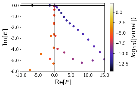
It is finally used to plot the Siegert states of all the potential with the same scale of virial values for the various potentials:

data_kwd = 'energies'
# Uncomment the next line to plot the wavenumbers
# data_kwd = 'wavenumbers'
if data_kwd == 'energies':
    re_lim = re_e_lim
    im_lim = im_e_lim
elif data_kwd == 'wavenumbers':
    re_lim = re_k_lim
    im_lim = im_k_lim
basissets = [basis1, basis2, basis3]
scatter_plot(data_kwd, basissets, show_unknown=False,
             xlim=re_lim, ylim=im_lim)

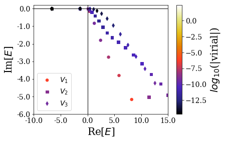
This shows that the spectrum of resonant states can vary greatly while the bound states are not very different. These differences can be caused by the distance between the two wells (which tend to stabilize more resonant states close to the threshold energy \(E=0\)) or by the presence of barriers (which creates quasi-bound states, which are nothing but very stable resonant states).

The energy of the lowest Siegert states is also presented in the following table:

# Print the header of the table
header = "   phi   |"
for i in range(len(basissets)):
    header += "|       V{}      ".format(i+1)
print(header)
print("-"*len(header))
# Print the table:
# - first, the bound states
bnd_energies = np.array([[en for en in np.sort(basis.bounds.energies)]
                         for basis in basissets])
for i in range(len(bnd_energies.T)):
    line = " phi_b_{} |".format(i+1)
    for en in bnd_energies.T[i]:
        line += "| {: .3f} ".format(en)
    print(line)
# - then, the resonant states
n_res = 5
res_energies = np.array([[en for en in np.sort(basis.resonants.energies[:n_res])]
                         for basis in basissets])
for i in range(n_res):
    line = " phi_r_{} |".format(i+1)
    for en in res_energies.T[i]:
        line += "| {: .3f} ".format(en)
    print(line)

   phi   ||       V1      |       V2      |       V3
----------------------------------------------------------
 phi_b_1 || -6.636+0.000j | -6.636+0.000j | -6.635+0.000j
 phi_b_2 || -6.636-0.000j | -6.636+0.000j | -6.635+0.000j
 phi_b_3 || -1.404-0.000j | -1.391+0.000j | -1.376+0.000j
 phi_b_4 || -1.377-0.000j | -1.391+0.000j | -1.347+0.000j
 phi_r_1 ||  0.381-0.156j |  1.376-0.395j |  1.149-0.035j
 phi_r_2 ||  1.270-0.833j |  2.074-0.688j |  1.775-0.122j
 phi_r_3 ||  2.439-1.802j |  2.837-1.038j |  2.627-0.286j
 phi_r_4 ||  3.922-2.764j |  3.651-1.373j |  3.661-0.568j
 phi_r_5 ||  5.872-3.810j |  4.587-1.642j |  4.809-0.959j