Defining a new symbolic potential

In this notebook, we’ll focus on the possibility of easily studying other symbolic potentials rather than on the physical information gained from the presented results. This is made possible thanks to the SymbolicPotential class, which is actually the base class for the WoodsSaxonPotential, TwoGaussianPotential and FourGaussianPotential classes.

Initialization

The SymbolicPotential class is imported from SiegPy:

import numpy as np
import matplotlib.pyplot as plt
from siegpy import SymbolicPotential, Hamiltonian, UniformCoordMap

A simple example

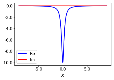
This potential is of the form \(-\frac{a}{x^2+b}\). The simplest way of initializing a symbolic potential is by defining a string where "x" is the only variable (all the parameters must be evaluated in the string). Another possibility is by directly using the sympy module to define a symbolic function (where x is the only allowed variable, or symbol).

# Define a grid
xmax = 9.0
xgrid = np.linspace(-xmax, xmax, 1001)
# Define the symbolic function as a string
a = 1
b = 0.1
sym_func = "-{} / (x**2 + {})".format(a, b)
# Initialize the ymbolic potential and plot it
pot = SymbolicPotential(sym_func, grid=xgrid)
pot.plot()

From there, the usual way of finding the eigenstates and plotting the results can be achieved:

cm = UniformCoordMap(0)
ham = Hamiltonian(pot, cm)
basis = ham.solve()

basis.plot_energies(xlim=(-10, 5), ylim=(-5, 1))
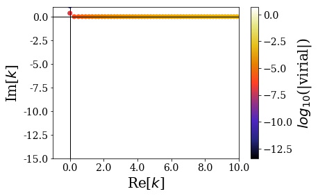
basis.plot_wavenumbers(xlim=(-1, 10), ylim=(-15, 1))
basis.plot_wavefunctions(nstates=3)

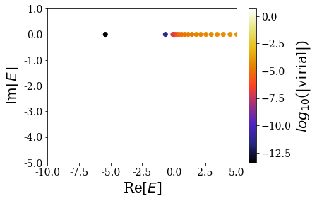
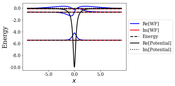
Note how this potential has a bound state close to the 0 energy: this state might require a more extended grid to be considered as converged.