Symbolic Woods-Saxon potential

The Square-Well Potential (SWP) used in all the previous notebooks can actually be considered as a Woods-Saxon Potential (WSP) with an infinitely large sharpness parameter.

In this notebooks, we will therefore obtain the resonant states of multiple WS potentials of varying sharpness parameters and compare the obtained spectra with the one obtained with the SW potential that corresponds to the infinite sharpness parameter.

Initialization

Some more lines are required for matplotlib because a plotting function will be defined in the end of the notebook. The class describing the Woods-Saxon potential is also imported from SiegPy.

import numpy as np
import matplotlib.pyplot as plt
import matplotlib.colors
from matplotlib import cm
from siegpy import (SWPotential, Hamiltonian, BasisSet,
                    ErfKGCoordMap, WoodsSaxonPotential)

Smooth potential

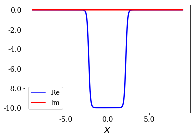
The first Woods-Saxon potential has the smallest sharpness parameter considered in this notebook, and is discretized over a grid.

# Define a grid
xmax = 9.0
xgrid = np.linspace(-xmax, xmax, 1201)
# Define the parameters of the first Woods-Saxon potenti
V0 = 10
l = np.sqrt(2)*np.pi
lbda1 = 4
# Definition of the first Woods-Saxon potential
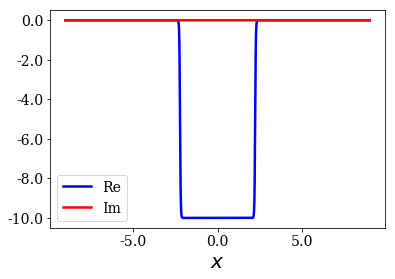
sym_pot_ws1 = WoodsSaxonPotential(l, V0, lbda1, grid=xgrid)
sym_pot_ws1.plot()

This potential is then used to define a Hamiltonian that is finally solved.

# Definition of the Hamiltonian to find the resonant states of this potential
cm_ws = ErfKGCoordMap(np.pi/4, xmax-1.5, 1.0)
ham_ws1 = Hamiltonian(sym_pot_ws1, cm_ws)
basis_ws1 = ham_ws1.solve(max_virial=10**(-3))

Let us finally look at some plots:

# Definition of all the parameters to get consistent plots for
# all the potentials considered throughout this notebook
re_e_max = 21
im_e_min = -13
im_k_max = np.sqrt(2*V0)
re_k_max = np.sqrt(2*re_e_max)
re_e_lim = (-V0, re_e_max)
im_e_lim = (im_e_min, -im_e_min/30)
re_k_lim = (-re_k_max/30, re_k_max)
im_k_lim = (-im_k_max, im_k_max)
# Plot the energies, wavenumbers and some eigenstates of the potential
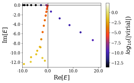
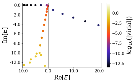
basis_ws1.plot_energies(xlim=re_e_lim, ylim=im_e_lim)
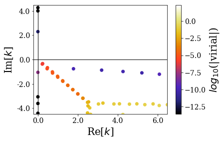
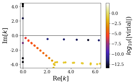
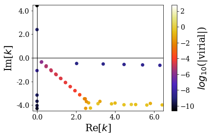
basis_ws1.plot_wavenumbers(xlim=re_k_lim, ylim=im_k_lim)
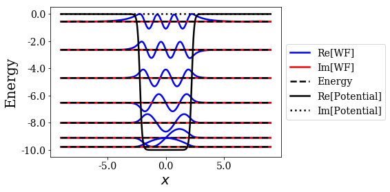
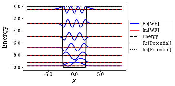
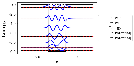
basis_ws1.plot_wavefunctions(nstates=7)

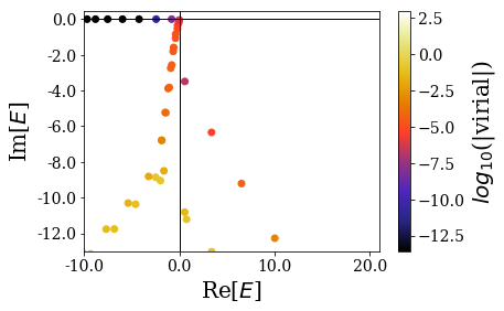
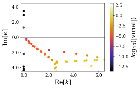
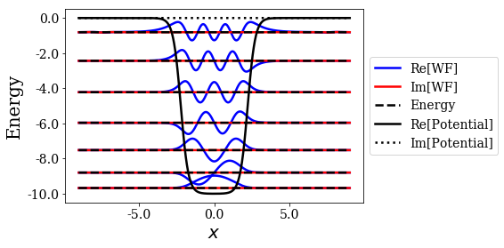
Bound states are found, and they seem rather similar to the ones found for the Square-Well potential, with low virial values. On the other hand, the resonant states are more difficult to find because the values of the imaginary part of their energy is high (in absolute value), so that it requires a large complex scaling angles. It is therefore not surprising they have rather high virial values, not so far away from those of the rotated continuum states.

Sharper potential

Let us now consider the case of a sharper potential:

# A larger sharpness parameter gives a sharper potential.
# All the other parameters are the same as in the previous case.
lbda2 = 10
sym_pot_ws2 = WoodsSaxonPotential(l, V0, lbda2, grid=xgrid)
sym_pot_ws2.plot()

The new potential is used to define another Hamiltonian, that is finally solved:

ham_ws2 = Hamiltonian(sym_pot_ws2, cm_ws)
basis_ws2 = ham_ws2.solve(max_virial=10**(-6))

Let us look at some plots:

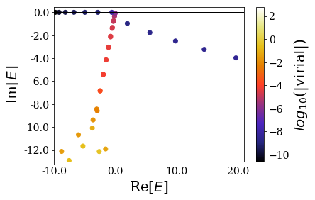
basis_ws2.plot_energies(xlim=re_e_lim, ylim=im_e_lim)
basis_ws2.plot_wavenumbers(xlim=re_k_lim, ylim=im_k_lim)
basis_ws2.plot_wavefunctions(nres=0)

This time, the resonant states are more easily found from the rest of the eigenstates: their imaginary value is closer to the axis \(\text{Im}[E] = 0\), and it would therefore require a lower complex scaling angle than in the previous case. Note that the virial values are also smaller for the resonant states, compared to the previous case.

Sharp potential

The last Woods-Saxon that will be considered will be even sharper:

# The sharpness parameter is increased again
lbda3 = 50
sym_pot_ws3 = WoodsSaxonPotential(l, V0, lbda3, grid=xgrid)
sym_pot_ws3.plot()

A new Hamiltonian is created, and it is solved again, allowing the production of more plots:

ham_ws3 = Hamiltonian(sym_pot_ws3, cm_ws)
basis_ws3 = ham_ws3.solve(max_virial=10**(-6))

basis_ws3.plot_energies(xlim=re_e_lim, ylim=im_e_lim)
basis_ws3.plot_wavenumbers(xlim=re_k_lim, ylim=im_k_lim)
basis_ws3.plot_wavefunctions(nres=0)

Again, it can be seen that the resonant states of this sharp potential have lower imaginary part of energy (in absolute value) than for the previous two potentials. They also have lower virial values.

Square-Well Potential

Let us now study the case of the Square-Well potential that is the limiting case of the Woods-Saxon potentials presented above, in the limit where the sharpness parameter is infinitely large:

# The same width, depth and grid is used
sw_pot = SWPotential(l, V0, grid=xgrid)
ham_sw = Hamiltonian(sw_pot, cm_ws)
basis_sw = ham_sw.solve(max_virial=10**(-6))

basis_sw.plot_energies(xlim=re_e_lim, ylim=im_e_lim)
basis_sw.plot_wavenumbers(xlim=re_k_lim, ylim=im_k_lim)
basis_sw.plot_wavefunctions(nres=0)

This is not different from all the plots obtained in the previous notebooks. The states that are obtained seem close to those of the sharper Woods-Saxon Potential considered, which is not that surprising. One detail still has to draw the attention: the virial values are much higher in this case.

Comparison of all the results

Siegert states and virial values

In order to plot only the bound and resonant states of all the basis sets while using only one scale for the virial, a new function has to be defined:

def scatter_plot(data_kwd, basissets, xlim=None, ylim=None, title=None,
                 file_save=None, show_unknown=False):
    # Object-oriented plots
    fig = plt.figure()
    ax = fig.add_subplot(111)
    # Add the real and imaginary axes
    ax.axhline(0, color='black', lw=1)  # black line y=0
    ax.axvline(0, color='black', lw=1)  # black line x=0
    # Define the min and max values of the virial, in order to
    # use the same normalized scale of for the virial values.
    allstates = BasisSet()
    for b in basissets:
        allstates += b
    vmin = np.min(np.log10(allstates.virials))
    vmax = np.max(np.log10(allstates.virials))
    norm = matplotlib.colors.Normalize(vmin=vmin, vmax=vmax)
    # Define the markers used for each basis set (not more than four
    # basis sets can be considered ; you can still add more markers here,
    # but the plot might become difficult to read)
    markers = ["o", "s", "d", "^"]
    # Loop over the basis sets to plot them
    for i, b in enumerate(basissets):
        # Select which states have to be plotted and store their virial
        to_plot = b.bounds + b.resonants + b.continuum
        if show_unknown is True or len(b.unknown) == len(b):
            to_plot += b.unknown
        virials = np.log10(to_plot.virials[::-1])
        # Set the x-axis label and get the data to be plotted, according
        # to the value of data_kwd.
        if data_kwd == 'wavenumbers':
            data_label = 'k'
            plot_data = to_plot.wavenumbers[::-1]
        elif data_kwd == 'energies':
            data_label = 'E'
            plot_data = to_plot.energies[::-1]
        # Else: raise a value error
        else:
            raise ValueError("data_kwd must be equal to 'wavenumbers' "
                             "or 'energies' (here '{}')".format(data_kwd))
        # Plot all the data
        if plot_data != []:
            # normalized scale for the colors
            c = plt.cm.CMRmap(norm(virials))
            ax.scatter(np.real(plot_data), np.imag(plot_data), c=c,
                       marker=markers[i], s=30, label="$V_{}$".format(i+1))
    # Set the colorbar and its title
    m = cm.ScalarMappable(cmap=plt.cm.CMRmap, norm=norm)
    m.set_array([])
    plt.colorbar(m, label="$log_{10}$(|virial|)")
    # Set axis labels and range and the plot title
    ax.set_xlabel("Re[${}$]".format(data_label))
    ax.set_ylabel("Im[${}$]".format(data_label))
    if xlim is not None:
        ax.set_xlim(xlim)
    ax.set_xticklabels(ax.get_xticks())
    if ylim is not None:
        ax.set_ylim(ylim)
    ax.set_yticklabels(ax.get_yticks())
    if title is not None:
        ax.set_title(title)
    plt.legend()
    # Save the plot and show it
    if file_save is not None:
        fig.savefig(file_save)
    plt.show()

This new function is finally used to plot the most interesting states:

data_kwd = 'energies'
# Uncomment the next line to plot the wavenumbers
# data_kwd = 'wavenumbers'
if data_kwd == 'energies':
    re_lim = re_e_lim
    im_lim = im_e_lim
elif data_kwd == 'wavenumbers':
    re_lim = re_k_lim
    im_lim = im_k_lim
basissets = [basis_ws1, basis_ws2, basis_ws3, basis_sw]
scatter_plot(data_kwd, basissets, show_unknown=False,
             xlim=re_lim, ylim=im_lim)

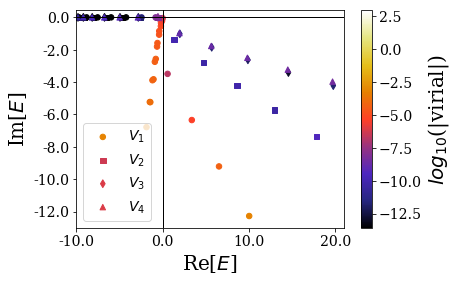
\(V_1\) (resp. \(V_2\) and \(V_3\)) corresponds to the first (resp. second and third) Woods-Saxon potential, while \(V_4\) corresponds to the SW potential. The trend for the resonant states is clearly visible, along with the fact that the virial values of the SWP are smaller than for the sharper Woods-Saxon potential, while their energy almost coincides. Note that it is clear that the resonant states of the smoothest potential are more difficult to separate from the rest of the rotated continuum states.

From there, it is clear that the smoother the Woods-Saxon potential, the higher the absolute value of the imaginary part of the resonant states energies: this means that it will be more difficult to identify the resonant states for smooth potentials, and that the resonant states of smooth potentials would also have very short lifetime (that is proportional to the absolute value of the imaginary part of the resonant state energy).

Focus on the bound states

Let us focus on the bound states energies found for all the potentials studied above. It will also be interesting to compare with the analytical results for the 1D Square-Well potential:

# Find the analytical Siegert states of the SWP (here, read from a file)
exact_siegerts = BasisSet.from_file("siegerts.dat")

The energies of the bound states for each basis set (i.e., for each potential) are represented in the following plot:

# Plot the bound states
basissets = [basis_ws1, basis_ws2, basis_ws3, basis_sw, exact_siegerts]
for i, basis in enumerate(basissets):
    bounds = BasisSet(states=basis.bounds[:7])
    plt.scatter([i+1]*len(bounds), np.real(bounds.energies), marker="_", s=2500)
plt.xlim(0.5, len(basissets)+0.5)
plt.xlabel("Potential $V_i$")
plt.ylabel("Re[Energy]")
plt.show()

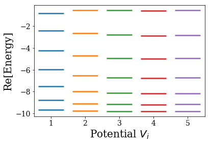
In this plot, \(V_5\) corresponds to the analytical SWP case. It is worth noting that the smoother potential has a more compact spectrum of bound states: the low energy bound states tend to be higher than those of the sharper potentials (because the potential width is smaller in this energy range), while the very high energy bound states tend to be more bound (because the potential has a larger width for such an energy range). We also see that the results converge to the analytical SW potential ones.

Another way to look at the energy of the bound states found for each potential is print them in a table. This is done below:

# Maximal number of states
i_max = 7
# Print the header of the table
header = " phi  |"
for i in range(len(basissets)):
    header += "|       V{}      ".format(i+1)
print(header)
print("-"*len(header))
# Print the table
energies = np.array([[en for en in np.sort((basis.siegerts).energies[:i_max])]
                     for basis in basissets])
for i in range(i_max):
    line = "phi_{} |".format(i+1)
    for en in energies.T[i]:
        line += "| {: .3f} ".format(en)
    print(line)

 phi  ||       V1      |       V2      |       V3      |       V4      |       V5
---------------------------------------------------------------------------------------
phi_1 || -9.674-0.000j | -9.774-0.000j | -9.793+0.000j | -9.795+0.000j | -9.794+0.000j
phi_2 || -8.795-0.000j | -9.103+0.000j | -9.173+0.000j | -9.181-0.000j | -9.177+0.000j
phi_3 || -7.519-0.000j | -8.007+0.000j | -8.147+0.000j | -8.163-0.000j | -8.154+0.000j
phi_4 || -5.960+0.000j | -6.523-0.000j | -6.725-0.000j | -6.753-0.000j | -6.737+0.000j
phi_5 || -4.224+0.000j | -4.702-0.000j | -4.930-0.000j | -4.970-0.000j | -4.945+0.000j
phi_6 || -2.435-0.000j | -2.635+0.000j | -2.811+0.000j | -2.859+0.000j | -2.826+0.000j
phi_7 || -0.809+0.000j | -0.555-0.000j | -0.539-0.000j | -0.581-0.000j | -0.545+0.000j

Conclusions

We presented the use of the Woods-Saxon potential in SiegPy and compared the Siegert states obtained when varying the sharpness of the potential, with the Square-Well potential case as a limit of an infinite sharpness parameter.

Obtaining the numerical resonant states of the smoother potential proves to be more difficult because their energies have imaginary parts that get higher (in absolute value). This means that large complex scaling angles have to be used, while the virial values obtained are very small compared to sharper potentials. However, if the potential is too sharp, the virial values are higher. It was also possible to see how the numerical bound states obtained converge to the ones of the SW potential when the sharpness parameter is increased.